Finding the Yellow Line
This was a project I did a while back, but it’s cool, and I haven’t written about it yet. Recently, several car manufacturers have started including a warning system to yell at you if you start drifting out of your lane.
I implemented a version of this that takes in video from the front of the car and continually tracks the geometric center of the lane marker. It doesn’t use OpenCV or any other vision libraries, just simple chromatic and density filtering and blob detection. Some of the code I’ll present here refer to data structures and memory allocations that are generated in other files. I think that stuff is kind of boring and it’s not too important for what I’m trying to show, that is, the general approach to this problem. The comments in the code should help clear up confusion, and I’ll highlight the important parts.
Chromatic Filtering
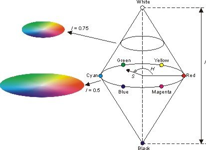
Chromatic filtering was performed in an integer HSI representation. It models RGB pixels with hue, saturation, and intensity. People often get confused between hue, saturation, and intensity, so here’s a good diagram that explains the differences:
Filtering an image based on chromaticity involves the hue and saturation values at every point. Depending on what you’re filtering for, thresholds must be empirically determined and set. It’s also a good idea to set limits on those parameters because low illumination in the image can cause erroneous hue and saturation values.
Here’s an example function that will replace an RGB value with an HSI value. It limits all fields to an 8 bit unsigned integer and replaces the vectored RGB pixel with the resulting HSI value. It returns that value in frame.
void RGB2HSIin(Pixel *P) {

unsigned char Max = P->R, Mid = P->G, Min = P->B, Delta;

if (Mid > Max) {
Mid ^= Max;
Max ^= Mid;
Mid ^= Max;
  }
if (Min > Mid) {
Min ^= Mid;
Mid ^= Min;
Min ^= Mid;
if (Mid > Max) {
Mid ^= Max;
Max ^= Mid;
Mid ^= Max;
  }
 }
Delta = Max - Min;
if (Max == 0) // black pixel
P->R = P->G = P->B = 0;
else if (Delta == 0) { // gray pixel
P->R = P->G = 0;
P->B = (Max + Mid + Min) / 3;
} else {
if (P->R == Max)
P->R = ((P->G - P->B) * 42 / Delta) + 42; // range from 0 - 84
else if (P->G == Max)
P->R = ((P->B - P->R) * 42 / Delta) + 127; // range from 85 - 169
else
P->R = ((P->R - P->G) * 42 / Delta) + 212; // range from 170 - 254
P->G = Delta * 255 / Max;
P->B = (Max + Mid + Min) / 3;
  }
}
You can do something similar to build a hue filter, but since it’s basically searching the image space for thresholds, I won’t reproduce the code here.
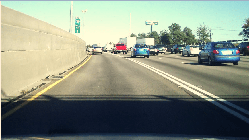
Here’s what that filter looks like when applied to an actual image. This is a single frame pulled from video footage taken from the dashboard of a car on the highway in Atlanta:
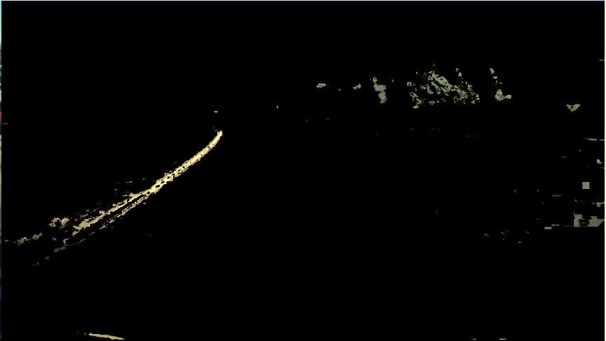
And here’s that same frame with a chromatic filter applied to look for the shade of yellow that the left lane marker is:
It’s clear that there are several parts of the image that are showing false positives for that shade of yellow. We’ll need to deal with that by running this through another filter.
Density Filtering
Density filtering essentially finds the areas of the image that have clusters of pixels we think are interesting. In this case, after chromatic filtering, only non-black pixels are interesting. We want to find the area image density. The following function will two dimensionally scan an input frame containing salient regions with blackened pixels everywhere else. It returns a preallocated map of contiguous salient pixels. You’ll see mentions of wheels here, that’s a metaphor for rolling the routine across the image.
void Area_Image_Density(FrmBuf *FB, int *DensityMap, int WheelSize) {

   int Wheels[FB->Height];
   int Sums[FB->Height];
   int Vwheel[WheelSize];
   int Vsum, Vptr, HalfWheel, WheelOff, X, Y, I, Edge;
   // initialize one in left edge of window
   Edge = 1 << (int) (WheelSize - 1);
   // half wheel size
   HalfWheel = WheelSize >> 1;
   // window offset = half window size x Width
   WheelOff = HalfWheel * (FB->Width + 1);
   for (Y = 0; Y < FB->Height; Y++) {  // for all rows
      Wheels[Y] = 0; // clear the wheels
      Sums[Y] = 0;   // clear the sums
   }
   // for each column plus write out rows
   for (X = 0; X < FB->Width + HalfWheel; X++) {
      // for all positions in vertical wheel
      for (Vptr = 0; Vptr < WheelSize; Vptr++)
         Vwheel[Vptr] = 0; // clear vertical wheel
      Vsum = Vptr = 0; // clear vertical sum and ptr
      // for each row
      for (Y = 0; Y < FB->Height + HalfWheel; Y++) {
       I = X + Y * FB->Width; // compute index
       Sums[Y] -= Wheels[Y] & 1; // remove outgoing pixel count
       Wheels[Y] >>= 1;  // shift window for new pixel
      Vsum -= Vwheel[Vptr];//removing outgoing vertical wheel count
         if (Y < FB->Height) { // while in image column
	    if (X < FB->Width ) // while in image row
               // if pixel contains non-blackened value
               if (FB->Frm[3*I] | FB->Frm[3*I+1] | FB->Frm[3*I+2]) {
	      Sums[Y] += 1; // increment count
	      Wheels[Y] |= Edge; // and insert new edge pixel count
               }
        Vwheel[Vptr] = Sums[Y]; // insert row sum on vertical wheel
            Vsum += Sums[Y]; // and add to vertical sum
         }
         Vptr = (Vptr + 1) % WheelSize; // increment vertical ptr
         // wait until fully into row and column
         if (X >= HalfWheel && Y >= HalfWheel)
	    // write current vertical sum to density map
            DensityMap[I - WheelOff] = Vsum;
      }
   }
}
If you wanted to, you could reverse the scan order of this function to take advantage of spacial locality in the cache and eek a little more speed out.
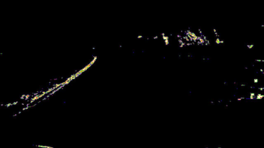
Here’s what running a chromatically filtered image through this density filter looks like:
Now that we’ve identified areas of interest, we look for features.
Blob Detection
Blob detection is again mostly a game of thresholds. The worst part of this whole project was playing with thresholds until stuff worked well enough. To find a blob, we compare the density of the image at a certain point to a threshold. If it is touching another blob, we combine those two into a single blob. Here’s a function that returns a list of blobs found in a given density map. It annotates all density map values with pointers to the corresponding blob. After scanning the map and identifying blobs, it flattens the map by forwarding points until a non-forwarded blob is found, and it’s ID is used to replace the blob pointer in the blob map.
Blob *Blob_Finder_Map(int *DensityMap, int Width, int Height, int Bth) {

   Blob *Blobs = NULL, *RowBlob;
   Blob *ColBlobs[Width];
   int  X, Y, I = 0;

   for (X = 0; X < Width; X++) // for all columns
      ColBlobs[X] = NULL; // clear column blobs
   for (Y = 0; Y < Height; Y++) { // for each row
      RowBlob = NULL; // clear row blob
      for (X = 0; X < Width; X++) { // for each row offset
         // if column blob is a fwd ptr
         if(ColBlobs[X] && ColBlobs[X]->FP)
          // then reduce to the vectored blob
	  ColBlobs[X] = Reduce_FP(ColBlobs[X]);
         if (DensityMap[I] >= Bth) { // if blob-worthy
	    if (RowBlob && ColBlobs[X]) // if two blobs touch
                // then merge column blob into rowblob
	       Merge_Blobs(ColBlobs[X], RowBlob, 0);
            else if (ColBlobs[X]) // if only column blob exists
	       RowBlob = ColBlobs[X]; // copy to row blob
            else if (RowBlob == NULL) { // if no current blobs
	       RowBlob = New_Blob(X,Y, 0); // allocate a new blob
               RowBlob->Next = Blobs;//push new blob onto blob list
               Blobs = RowBlob; // update blob list
            }
	 Add_Position(RowBlob, X, Y);//add position to current blob
            ColBlobs[X] = RowBlob; // update column blob
            // store blob address in blob map
	    DensityMap[I] = (int) RowBlob;
	 } else { // else leaving blob
	    // clear blob map for unblob-worthy positions
            DensityMap[I] = 0;
             // clear current blob pointers
	    RowBlob = ColBlobs[X] = NULL;
	 }
	 I += 1; // adjust map index
      }
   }
   Number_Blobs(Blobs); // set ID on non-forwarded blobs
   // transform blob pointers to base ID
   Mark_Blob_ID_Map(DensityMap, Width * Height);
   // eliminate residual fwd ptrs from last row
   Blobs = Reap_FP_Blobs(Blobs);
   // return blob list
   return (Blobs);
}
If you visualize those blobs by drawing squares around them, here’s what you get:
You can see that we picked up a bunch of blobs. To detect the yellow lane marker, you want to adjust all of those thresholds in each filter so that the largest blob contains the lane marker. When I ran this code, I would occasionally get two large blobs covering the lane marker. There are a lot of ways to try to detect the marker from this point, and most of them involve having a flexible algorithm and taking advantage of preexisting knowledge. For instance, you know that the marker will always be approximately a straight line, and it’s always going to be roughly diagonal as it moves towards the vanishing point. You also know that the line won’t do some things, like curve around backwards, spiral, get thicker, etc.
Here’s a video showing a bunch of different attempts at this problem. After the lane marker was detected, a line was drawn down the perceived middle of it. Each attempt is a different color. You can see that some are much better than others. Try to guess what parameter was wrong in different attempts.
2 Comments